Basic Computer Vision with CNNs

Author’s note: So this is a rather new topic, even though I have played around with dense (fully connected) networks before - convolutional networks are a new concept for me and I was surprised with its performance.

There’s certainly more I should be finding out about CNNs, but it’s gonna take a while so here’s a quick rundown of the simple - also just so I can quickly come back and review through this stuff later on. A content summary of stuff from chapter 14 of Hands-on Machine Learning (great practical book, I’m enjoying learning from it).

The Layers

Convolutional layer

In a traditional dense layer, every neuron in a layer is connected to the outputs of every neuron in the layer before it. This generally means, if we pass in an image to a dense layer, it tries to find a relationship between every pixel in the image, which as may be apparent is not how images work.

In an image, only some related pixels form a line or an edge, which in turn makes up a shape that our eyes and brain interprets as an object. It can be seen why a dense layer may not be appropriate for learning to identify images. That is where convolutional layers come in.

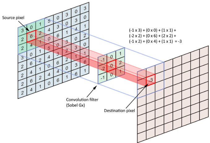
A convolutional layer is made up of stacked layers of filters. Each filter usually looks for different relationships in an image. In the example notebook below, there is a horizontal filter and a vertical filter, but a convolutional layer are made up of many more than just that.

Each filter is a matrix, generally described by a kernel size (how many pixels the filter processes at once), and is shifted through the image matrix performing matrix multiplication (dot product) between the filter kernel and the region of the image the kernel is over. The step size between each shift is determined by the stride. If there are multiple channels (e.g. RGB), the filter will perform those operations across all the channels.

In the above example, the two filters created have a 3x3 kernel size and the convolutional layer the filters are given to therefore have 2 filters (or feature maps) and a stride of 1. A convolutional layer is preferred over a fully connected layer in computer vision for its ability to reduce the image down into various features with spatial dependencies.

As can be seen then, the larger the kernel size, the more the image will be reduced. In larger images, the model may start with the largest kernel size (7x7) to reduce the input information down. Though in general, a 3x3 kernel size is most common. Meanwhile, the output size can be reduced using the size of the stride as well. A stride of 2 will essentially halve the output dimensions (or reduce area by 75%), as the filter is being shifted by 2 spots each time across the input.

To note, there is a “special” convolutional layer, which has a kernel size of 1x1. At first glance, it may seem that this layer wouldn’t do anything as it maps the output layer 1-to-1 directly. However, what a 1x1 convolutional layer can do is increase or decrease the number of feature maps in the input. This could be useful for reducing the dimensionality of the input and remove redundant filters or lower computational load. As such, a 1x1 kernel is usually placed before another convolutional layer.

A problem arises with each layer the image passes through though. For one, the outputs are shrinking, which may be undesirable if you want to maintain information across layers. The information on the outer edge of the image is processed less than that in the center and is being lost. The solution to this is to use zero padding, which is essentially adding a rim of 0s around the input (in keras, use padding='same'). This helps maintain the output size, which will only decrease when we specify it to, such as using a 2-stride.

I’ve largely been using Keras to create neural networks and that won’t change here, so creating a convolutional layer in keras can be done with keras.layers.Conv2D.

tf.keras.layers.Conv2D(
    filters,
    kernel_size,
    strides=(1, 1),
    padding="valid",
    data_format=None,
    dilation_rate=(1, 1),
    groups=1,
    activation=None,
    use_bias=True,
    kernel_initializer="glorot_uniform",
    bias_initializer="zeros",
    kernel_regularizer=None,
    bias_regularizer=None,
    activity_regularizer=None,
    kernel_constraint=None,
    bias_constraint=None,
    **kwargs
)

Pooling layer

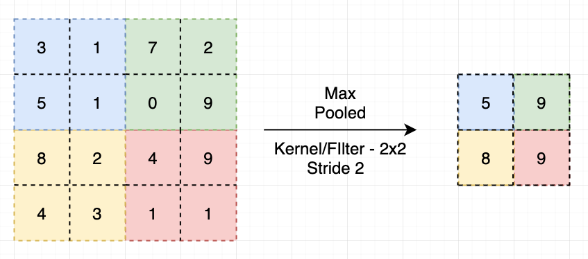
The responsibility of a pooling layer is to reduce the computational load and memory usage by subsampling (reduce) the image. Unlike a convolutional layer, a pooling layer has no weights; it only performs a function on the inputs (either max or mean or some other aggregation function). A pooling layer has a kernel size as well as a stride value. Typically, the stride is set to 2 to reduce the output dimensions by half. Also of note, the pooling layer performs its function on each channel independently.

The more popular pooling layer is the max pooling layer (as in the image above), which takes the maximum value within the kernel as the output value. There is also the average pooling layer though, which calculates the average of all the values in the kernel window.

Pooling layers also makes the model more invariant to changes. Say if certain features were shifted slightly in one direction, depending on the kernel size, the pooling layer may produce the same output. This is useful in classification tasks, where the location of the object does not matter.

In Keras, pooling layers are also available. One such is the MaxPooling2D.

tf.keras.layers.MaxPooling2D(
    pool_size=(2, 2), strides=None, padding="valid", data_format=None, **kwargs
)

There is also another frequently used pooling layer called the global average pooling layer, which calculates the mean of the values across each entire feature map. This is the same as using an average pooling layer with pool_size equal to the dimensions of the feature map. It is generally useful as an output layer. (In Keras, it is the GlobalAveragePooling2D layer)

Examples

I’ll just go into a couple of example models I’ve already trained and played with quite a bit.

Simple CNN

The following is a simple CNN trained on the MNIST handwritten numbers dataset.

The structure of the CNN can be seen in model.summary(), although I suppose it may be excessive for a simple dataset as MNIST. I will say, however, that this CNN model performs significantly better than I could get from a dense neural network (~85% accuracy).

The first convolutional layer creates 32 feature maps using a 7x7 kernel. Then, I double the feature maps every two layers after that, from 64 up to 256, each with a 3x3 kernel. Every layer is regularized with BatchNormalization and uses ReLU activation. The feature maps can be doubled as I reduce the dimensions by half with a max pooling layer.

Finally, as with typical simple CNNs the image goes through a couple of dense layers before being output using the softmax activation.

This simple CNN is likely most similar to AlexNet, which is a rather old model.

Transfer learning

For more complex models though, you can take a pretrained model without its final dense layers (i.e. only the convolutional layers), add your own dense layers and train it on your own data.

In the example, I used the Xception model available on Keras and trained it on the tf_flowers dataset. It is important to note that, for importing the model without the top dense layer, include_top=False. The pretrained models from Keras were trained on the ImageNet dataset (more info available here).

Also note, I used the Keras ImageDataGenerator class to create batches of training data, although it was largely moot here because the dataset isn’t that large (it was only to try it out). The Keras fit function now takes generators as well, since the original fit_generator function is deprecated as of TF 2.1.0+ (or something like that)

The Xception model uses several different techniques to improve performance, including residual blocks and, instead of inception modules from GoogleNet, depthwise separable convolution layer (which models spatial patterns and cross-channel patterns separately). I might go into a short post about the residual blocks (and ResNet, where they are from), especially since it’s not too complicated to understand and implement.

From here, there’s also the topic of semantic segmentation and object detection, of which I will look into some models more. The book I referenced and mentioned in at the very top doesn’t go into too much detail on this, so I’ll try looking into models like YOLOv3 and Fast-RCNN, both of which do object detection quite well.